AMOC Publication Figures

This notebook demonstrates how to create publication-quality AMOC figures using the AMOCatlas package with PyGMT. It reproduces plots similar to those in Frajka-Williams et al. (2019, 2023) and other AMOC publications.

Features:

• Clean, simplified workflow using amocatlas module functions

• Publication-quality PyGMT plots

• Multi-array time series comparison

• Tukey filtering for low-frequency analysis

• Component breakdown plots (e.g., RAPID, OSNAP)

Figures are designed to be re-used: the “AMOCatlas” badge and timestamp can be cropped out.

Suggested citation:

• For the multi-panel figure, you can say “updated from Frajka-Williams et al. 2019”.

import os

# AMOCatlas imports
from amocatlas import read, tools, plotters

# Set GMT library path if needed (adjust for your system)
# os.environ["GMT_LIBRARY_PATH"] = "/opt/homebrew/lib"  # macOS Homebrew
# os.environ["GMT_LIBRARY_PATH"] = "/usr/lib"          # Linux

# Create figures directory for documentation
figures_dir = "../docs/source/_static/paperfigs"
os.makedirs(figures_dir, exist_ok=True)
print(f"✓ Figures will be saved to: {figures_dir}/")

✓ Figures will be saved to: ../docs/source/_static/paperfigs/

1. Load and Standardize Data

Load MOC data from all major observing arrays and convert to standardized format.

# Load datasets
print("Loading AMOC array datasets...")

# RAPID 26°N
rapid_std = read.rapid(all_files=True)

# MOVE 16°N
move_std = read.move()

# OSNAP Subpolar
osnap_std = read.osnap(transport_only=True)

# SAMBA 34.5°S
samba_std = read.samba(all_files=True)

print("✓ All datasets loaded and standardized")

Loading AMOC array datasets...
Loading 5 RAPID 26°N dataset(s):
  0. moc_transports.nc: RAPID layer transport time series
  1. moc_vertical.nc: RAPID vertical streamfunction time series
  2. ts_gridded.nc: RAPID gridded temperature and salinity
  3. 2d_gridded.nc: RAPID 2D gridded data
  4. meridional_transports.nc: RAPID meridional transport data

Loading 1 MOVE 16°N dataset(s):
  0. OS_MOVE_20000206-20221014_DPR_VOLUMETRANSPORT.nc: MOVE transport time series

Loading 1 OSNAP dataset(s):
  0. OSNAP_MOC_MHT_MFT_TimeSeries_201408_202207_2025.nc: Time series of MOC, MHT, and MFT (2014-2022)

Loading 2 SAMBA 34.5°S dataset(s):
  0. Upper_Abyssal_Transport_Anomalies.txt: Daily volume transport anomaly estimates for the upper and abyssal cells of the MOC
  1. MOC_TotalAnomaly_and_constituents.asc: Daily travel time values, calibrated to a nominal pressure of 1000 dbar, and bottom pressures from the two PIES/CPIES moorings

✓ All datasets loaded and standardized

2. Extract Time Series to Pandas DataFrames

Convert xarray datasets to pandas DataFrames for filtering and PyGMT plotting.

# Extract time series using new tools functions
rapid_df = tools.extract_time_and_time_num(rapid_std[0])
rapid_df["moc"] = rapid_std[0]["MOC"].values

move_df = tools.extract_time_and_time_num(move_std)
move_df["moc"] = -move_std["MOC"].values  # Sign correction

osnap_df = tools.extract_time_and_time_num(osnap_std)
osnap_df["moc"] = osnap_std["MOC_SIGMA0"].values

samba_df = tools.extract_time_and_time_num(samba_std[1])  # Use dataset [1] for MOC
samba_df["moc"] = samba_std[1]["MOC"].values

print("Time series extracted:")
print(f"  RAPID: {len(rapid_df)} points")
print(f"  MOVE:  {len(move_df)} points")
print(f"  OSNAP: {len(osnap_df)} points")
print(f"  SAMBA: {len(samba_df)} points")

Time series extracted:
  RAPID: 14599 points
  MOVE:  4164 points
  OSNAP: 96 points
  SAMBA: 2964 points

3. Bin Data to Monthly Resolution

Ensure consistent temporal resolution across arrays for comparison.

# Bin to monthly resolution if needed
rapid_binned = tools.check_and_bin(rapid_df)
move_binned = tools.check_and_bin(move_df)
osnap_binned = tools.check_and_bin(osnap_df)
samba_binned = tools.check_and_bin(samba_df)

# Handle SAMBA temporal gaps to prevent plotting artifacts
samba_binned = tools.handle_samba_gaps(samba_binned)

print("✓ Data binned to consistent temporal resolution")
print("✓ SAMBA gaps handled to prevent plotting artifacts")

✓ Data binned to consistent temporal resolution
✓ SAMBA gaps handled to prevent plotting artifacts

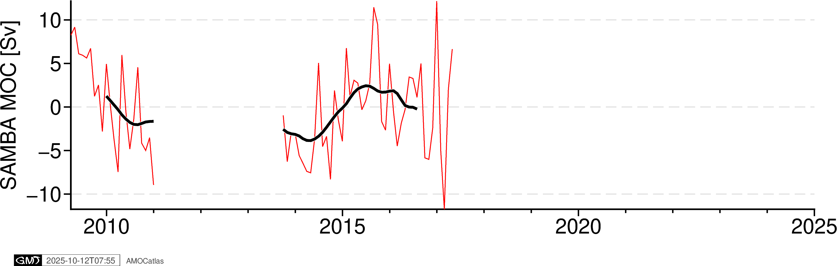
Special Handling for SAMBA Data

SAMBA MOC data contains significant temporal gaps (e.g., 2011-2014) that can cause plotting artifacts. PyGMT and other plotting functions connect all valid (non-NaN) data points regardless of temporal gaps, creating spurious lines across missing periods. The tools.handle_samba_gaps() function prevents these artifacts by:

1. Creating a regular monthly time grid

2. Preserving NaN values where no original data existed

3. Only allowing interpolation within continuous data segments

This ensures clean plots without false connections across data gaps.

4. Apply Tukey Filtering

Apply 18-month Tukey filter to highlight low-frequency variability.

# Apply 18-month Tukey filter for low-frequency analysis
filter_params = {"window_months": 18, "samples_per_day": 1/30, "alpha": 0.5}

rapid_filtered = tools.apply_tukey_filter(rapid_binned, column="moc", **filter_params)
move_filtered = tools.apply_tukey_filter(move_binned, column="moc", **filter_params)
osnap_filtered = tools.apply_tukey_filter(osnap_binned, column="moc", **filter_params)
samba_filtered = tools.apply_tukey_filter(samba_binned, column="moc", **filter_params)

print("✓ Tukey filtering applied (18-month window)")

✓ Tukey filtering applied (18-month window)

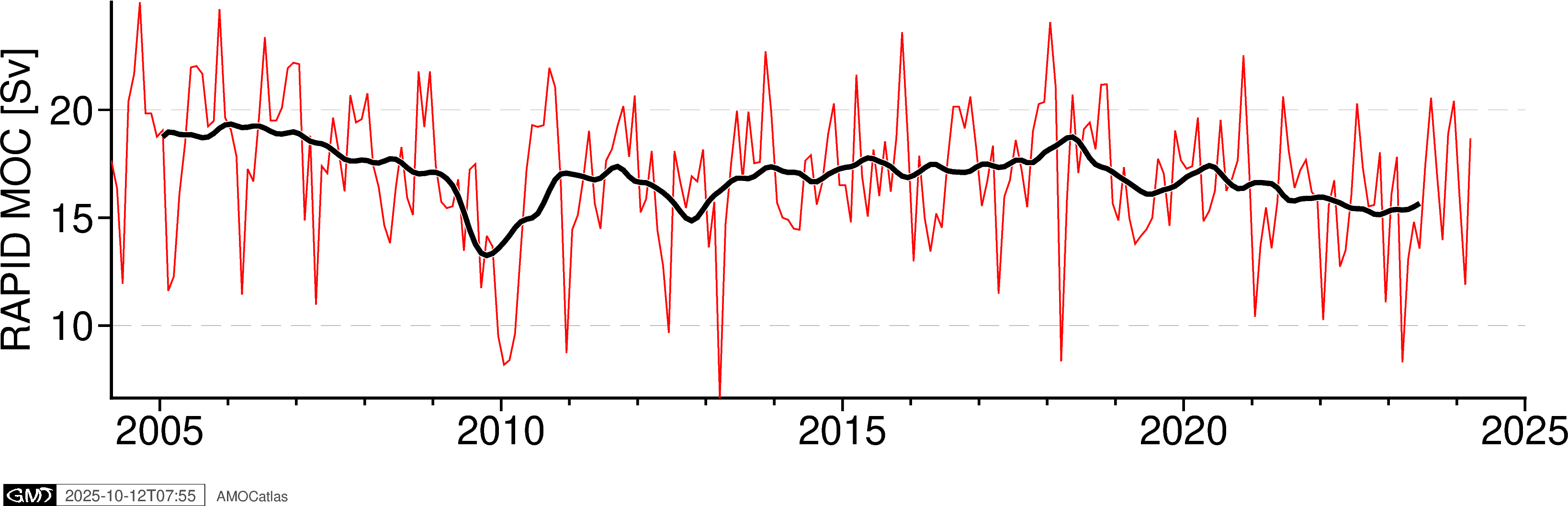
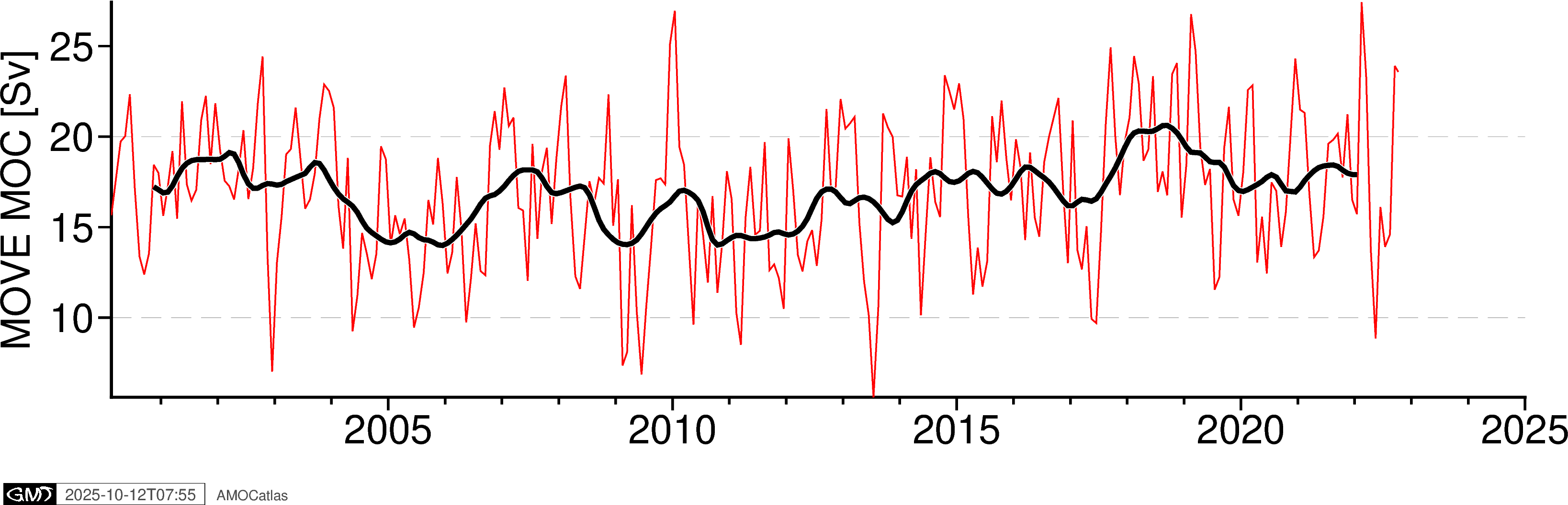
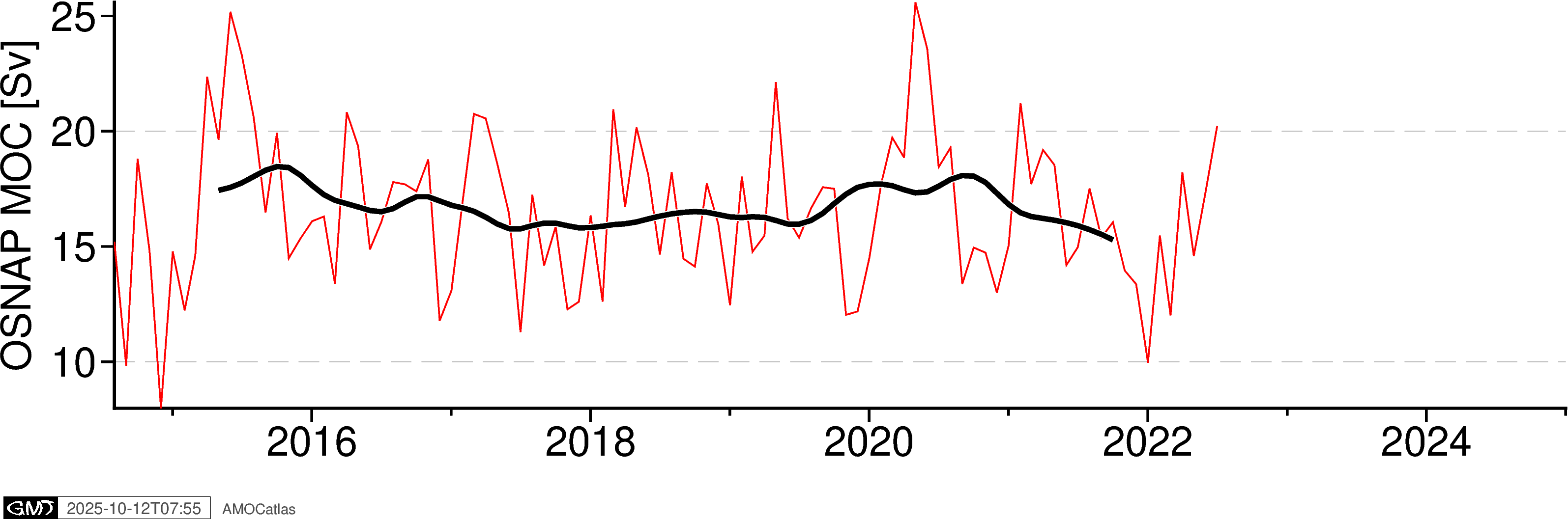
5. Single Array Time Series Plots

Create individual time series plots for each array.

# Individual time series plots
try:
    fig_rapid = plotters.plot_moc_timeseries_pygmt(rapid_filtered, label="RAPID MOC [Sv]")
    fig_rapid.show()

    fig_move = plotters.plot_moc_timeseries_pygmt(move_filtered, label="MOVE MOC [Sv]")
    fig_move.show()

    fig_osnap = plotters.plot_moc_timeseries_pygmt(osnap_filtered, label="OSNAP MOC [Sv]")
    fig_osnap.show()

    fig_samba = plotters.plot_moc_timeseries_pygmt(samba_filtered, label="SAMBA MOC [Sv]")
    fig_samba.show()

except ImportError as e:
    print(f"PyGMT not available: {e}")
    print("Install with: pip install pygmt")

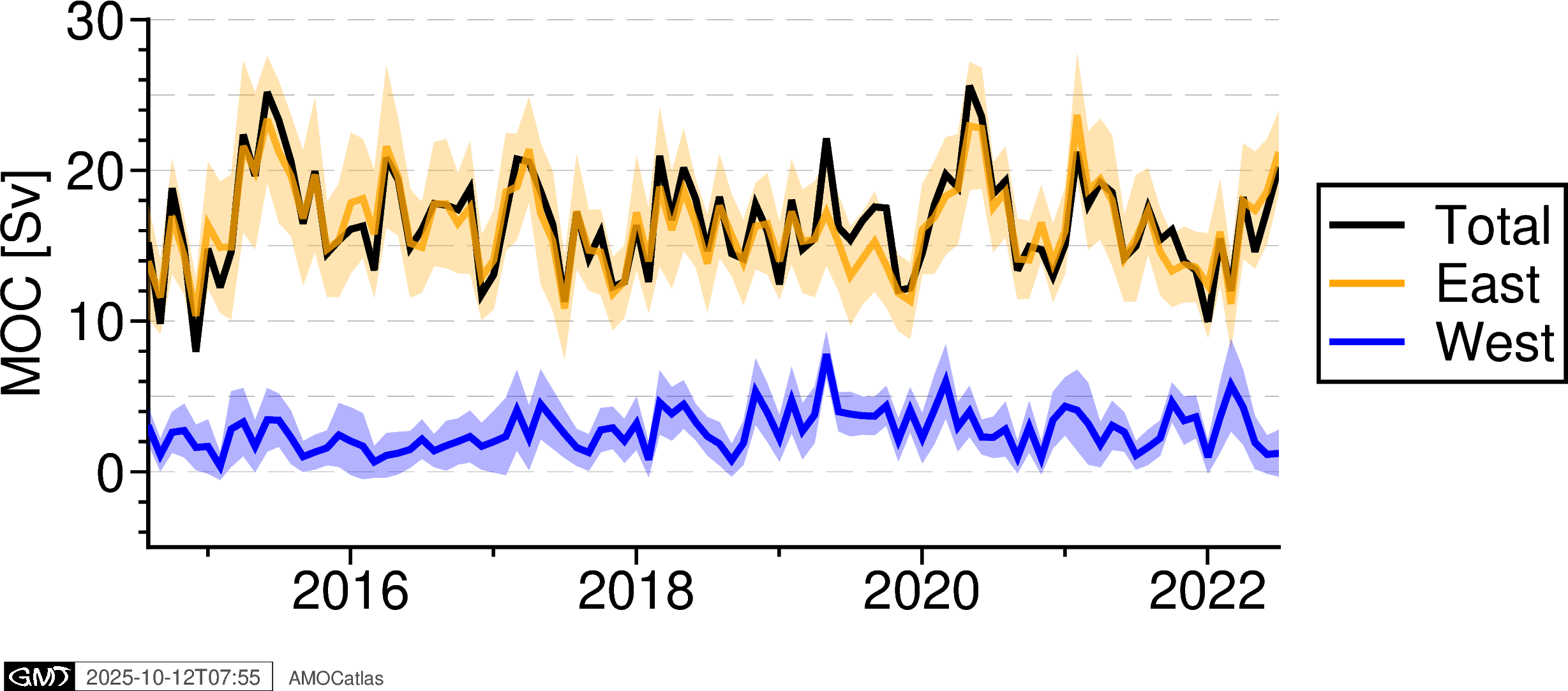
# OSNAP components plot with error bands
try:
    # Extract OSNAP component data
    ds = osnap_std
    osnap_components = tools.extract_time_and_time_num(ds)

    # Add all OSNAP variables
    for var in ["MOC_SIGMA0", "MOC_SIGMA0_ERR", "MOC_EAST_SIGMA0", "MOC_EAST_SIGMA0_ERR",
                "MOC_WEST_SIGMA0", "MOC_WEST_SIGMA0_ERR"]:
        osnap_components[var] = ds[var].values

    fig_osnap_comp = plotters.plot_osnap_components_pygmt(osnap_components)
    fig_osnap_comp.show()

    # Optional: save high-resolution version
    # fig_path = os.path.join(figures_dir, "osnap_components.png")
    # fig_osnap_comp.savefig(fig_path, dpi=300, transparent=True)
    # print(f"✓ Saved: {fig_path}")

except ImportError as e:
    print(f"PyGMT not available: {e}")

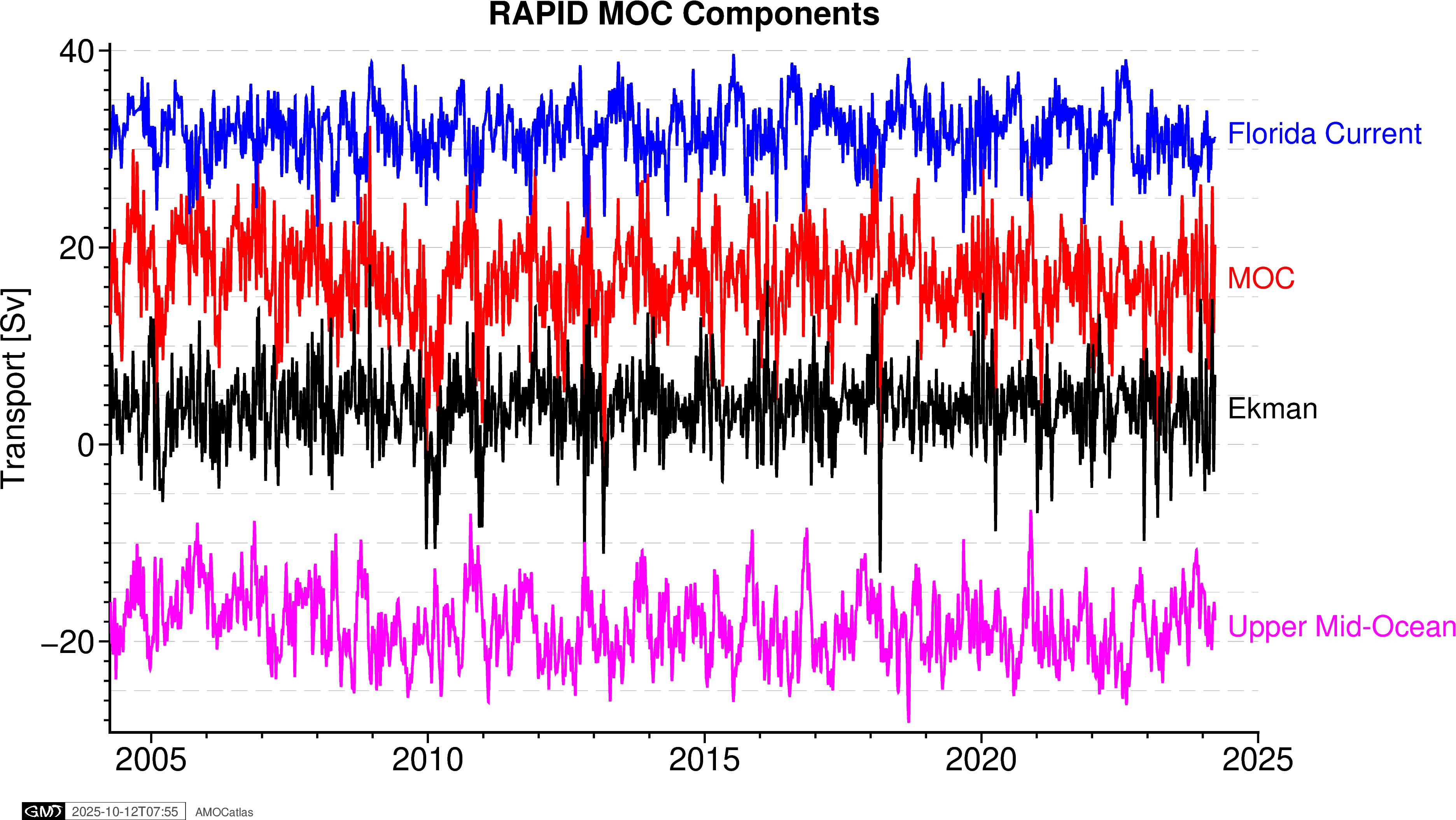
6. RAPID components plot

# RAPID components plot
try:
    # Extract RAPID component data
    ds = rapid_std[0]
    rapid_components = tools.extract_time_and_time_num(ds)

    # Add transport components
    rapid_components["moc_mar_hc10"] = ds["MOC"].values
    rapid_components["t_gs10"] = ds["TRANS_FC"].values  # Florida Current
    rapid_components["t_ek10"] = ds["TRANS_EKMAN"].values  # Ekman
    rapid_components["t_umo10"] = ds["TRANS_UMO"].values  # Upper Mid-Ocean

    fig_rapid_comp = plotters.plot_rapid_components_pygmt(rapid_components)
    fig_rapid_comp.show()

except ImportError as e:
    print(f"PyGMT not available: {e}")

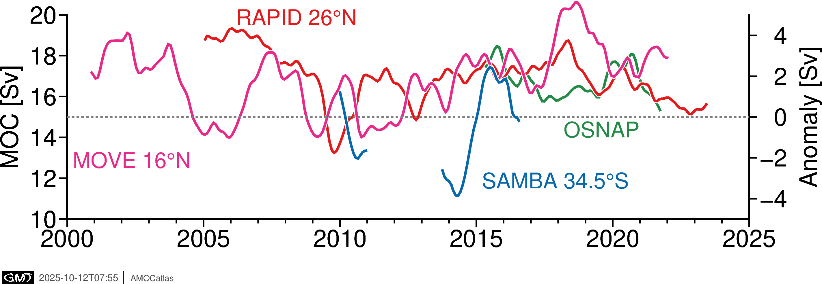
7. Multi-array comparison plot - original data

try: fig_multi = plotters.plot_all_moc_pygmt( osnap_filtered, rapid_filtered, move_filtered, samba_filtered, filtered=False ) fig_multi.show()

# Save high-resolution version
fig_path = os.path.join(figures_dir, "amoc_multi_array.png")
fig_multi.savefig(fig_path, dpi=300, transparent=True)
print(f"✓ Saved: {fig_path}")

except ImportError as e: print(f”PyGMT not available: {e}”)

# Multi-array comparison plot - filtered data
try:
    fig_multi_filt = plotters.plot_all_moc_pygmt(
        osnap_binned, rapid_binned, move_binned, samba_binned,
        filtered=False
    )
    fig_multi_filt.show()

    # Save high-resolution version
    fig_path = os.path.join(figures_dir, "amoc_multi_array.png")
    fig_multi_filt.savefig(fig_path, dpi=300, transparent=True)
    print(f"✓ Saved: {fig_path}")

except ImportError as e:
    print(f"PyGMT not available: {e}")

✓ Saved: ../docs/source/_static/paperfigs/amoc_multi_array.png

# Or overlaid, with SAMBA offset because it's an anomaly

fig_overlaid = plotters.plot_all_moc_overlaid_pygmt(
    osnap_filtered, rapid_filtered, move_filtered, samba_filtered,
    filtered=True
)

fig_overlaid.show()

## 8. Historical AMOC estimates from Bryden et al. 2005

try:
    fig_bryden = plotters.plot_bryden2005_pygmt()
    fig_bryden.show()

    # Save high-resolution version
    fig_path = os.path.join(figures_dir, "bryden2005_amoc.png")
    fig_bryden.savefig(fig_path, dpi=300, transparent=True)
    print(f"✓ Saved: {fig_path}")

except ImportError as e:
    print(f"PyGMT not available: {e}")

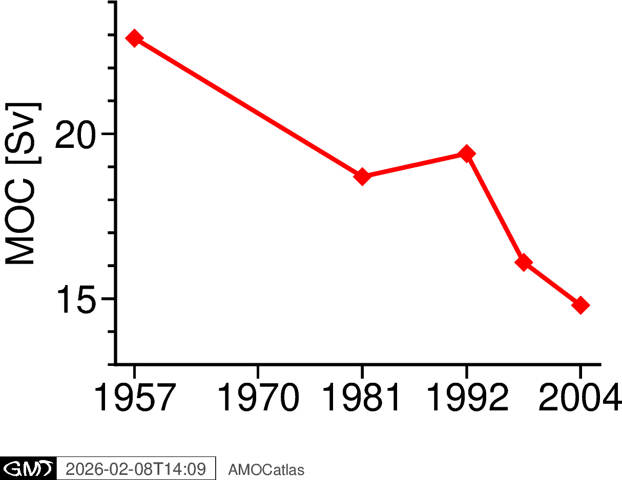
✓ Saved: ../docs/source/_static/paperfigs/bryden2005_amoc.png

9. Summary

This notebook demonstrates the streamlined workflow for creating publication-quality AMOC figures:

1. Data Loading: Using read.rapid() for consistent data access and standardisation

2. Time Series Processing: Converting to pandas with tools.extract_time_and_time_num()

3. Gap Handling: Using tools.handle_samba_gaps() to prevent plotting artifacts

4. Filtering: Applying Tukey filters with tools.apply_tukey_filter()

5. Visualization: Creating publication plots with plotters.plot_*_pygmt() functions

Key Features:

• Modular design using AMOCatlas functions

• Optional PyGMT dependency with graceful fallback

• Consistent styling across all plots

• Proper handling of temporal gaps in SAMBA data

• Historical context from Bryden et al. (2005)

• High-resolution export capability (saved to docs/source/_static/paperfigs/)