AMOCatlas demo
The purpose of this notebook is to demonstrate the functionality of AMOCatlas.
The demo is organised to show
Step 1: Loading and plotting a sample dataset
Step 2: Exploring the dataset attributes and variables.
Note that when you submit a pull request, you should clear all outputs from your python notebook for a cleaner merge.
[1]:
import pathlib
import sys
import os
from amocatlas import read, plotters

script_dir = pathlib.Path().parent.absolute()
parent_dir = script_dir.parents[0]
sys.path.append(str(parent_dir))

# Specify the path for writing datafiles
data_path = os.path.join(parent_dir, "data")
Load RAPID 26°N
To see what files are available for each data source, use read.DATASOURCE.list_files(). So for the RAPID array, you can use read.rapid.list_files().
You can then use this list (or a subset thereof) to specify which files to be loaded and standardised using the read.rapid(file_list=["file1", "file2"]) function with the input file_list. It will return a list of xarray datasets, in the same order and the same length as file_list. An exception is if file_list has length = 1, in which case it will return just the xarray dataset.
[2]:
# Find available files
rapid_file_list = read.rapid.list_files()

print("Available RAPID files:")
print(rapid_file_list)

# To specify to read two of those files, provide a file_list
standardRAPID = read.rapid(file_list = rapid_file_list[0:2])
Available RAPID files:
['moc_transports.nc', 'moc_vertical.nc', 'ts_gridded.nc', '2d_gridded.nc', 'meridional_transports.nc']
Loading 2 RAPID 26°N dataset(s):
  0. moc_transports.nc: RAPID layer transport time series
  1. moc_vertical.nc: RAPID vertical streamfunction time series
/home/runner/micromamba/envs/amocatlas/lib/python3.14/site-packages/xarray/backends/plugins.py:109: RuntimeWarning: Engine 'gmt' loading failed:
Error loading GMT shared library at 'libgmt.so'.
libgmt.so: cannot open shared object file: No such file or directory
  external_backend_entrypoints = backends_dict_from_pkg(entrypoints_unique)
[3]:
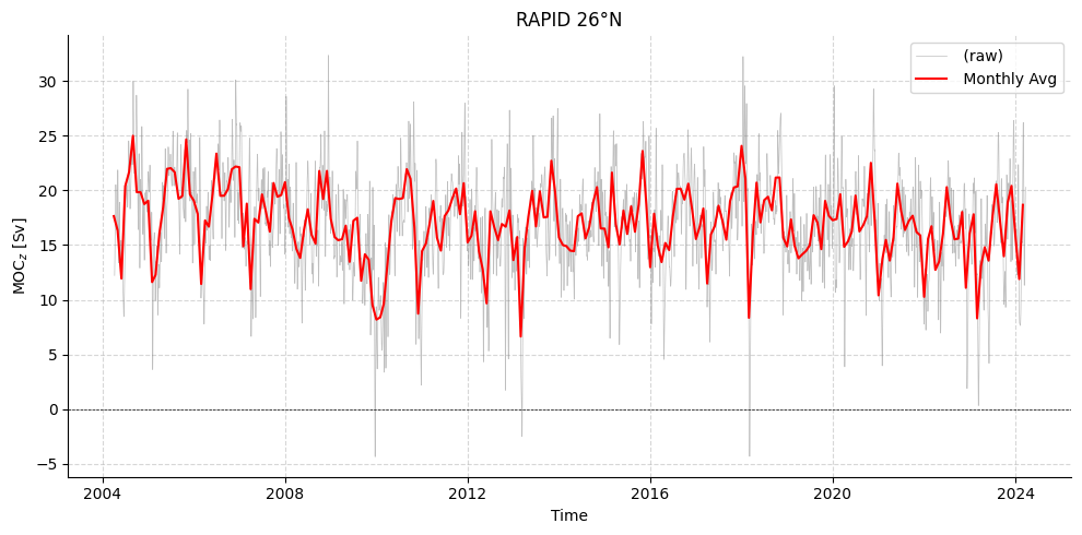
# Plot RAPID timeseries
plotters.plot_amoc_timeseries(
    data=[standardRAPID[0]],
    varnames=["MOC"],
    labels=[""],
    resample_monthly=True,
    plot_raw=True,
    figsize=(10, 5),
    title="RAPID 26°N"
)
[3]:
(<Figure size 1000x500 with 1 Axes>,
 <Axes: title={'center': 'RAPID 26°N'}, xlabel='Time', ylabel='MOC$_{z}$ (Sv)'>)
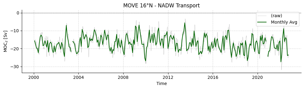
Load MOVE 16°N
To load the specified default transport file, use the read.DATASOURCE() function with no inputs. So for the MOVE array, this is read.move(). It will provide a single xarray dataset. For each array, a default transport file has been specified.
Developer’s note: This is specified in ~/amocatlas/data_source/DATASOURCE.py.
[4]:
ds_move = read.move()
Loading 1 MOVE 16°N dataset(s):
  0. OS_MOVE_20000206-20221014_DPR_VOLUMETRANSPORT.nc: MOVE transport time series
[5]:
# Plot MOVE timeseries
plotters.plot_amoc_timeseries(
    data=[ds_move],
    varnames=["MOC"],
    labels=[""],
    colors=["darkgreen"],
    resample_monthly=True,
    plot_raw=True,
    title="MOVE 16°N - NADW Transport"
)
[5]:
(<Figure size 1000x300 with 1 Axes>,
 <Axes: title={'center': 'MOVE 16°N - NADW Transport'}, xlabel='Time', ylabel='MOC$_{z}$ (Sv)'>)
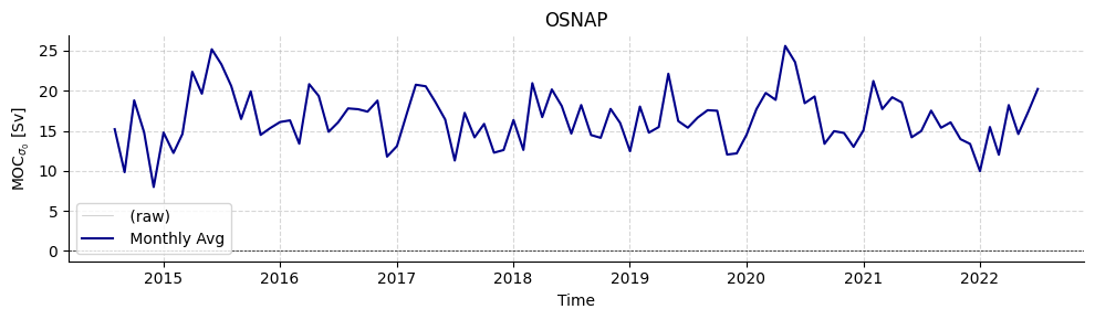
Load OSNAP
For just the transport file, you can use either read.osnap() as above, or read.osnap(transport_only=True). Both return a single xarray dataset.
[6]:
ds_osnap = read.osnap()
ds_osnap
Loading 1 OSNAP dataset(s):
  0. OSNAP_MOC_MHT_MFT_TimeSeries_201408_202207_2025.nc: Time series of MOC, MHT, and MFT (2014-2022)
[6]:
<xarray.Dataset> Size: 15kB
Dimensions:              (TIME: 96)
Coordinates:
  * TIME                 (TIME) datetime64[ns] 768B 2014-08-01T12:00:00 ... 2...
Data variables: (12/18)
    MOC_SIGMA0           (TIME) float64 768B ...
    MOC_SIGMA0_ERR       (TIME) float64 768B ...
    MOC_EAST_SIGMA0      (TIME) float64 768B ...
    MOC_EAST_SIGMA0_ERR  (TIME) float64 768B ...
    MOC_WEST_SIGMA0      (TIME) float64 768B ...
    MOC_WEST_SIGMA0_ERR  (TIME) float64 768B ...
    ...                   ...
    MFT                  (TIME) float64 768B ...
    MFT_ERR              (TIME) float64 768B ...
    MFT_EAST             (TIME) float64 768B ...
    MFT_EAST_ERR         (TIME) float64 768B ...
    MFT_WEST             (TIME) float64 768B ...
    MFT_WEST_ERR         (TIME) float64 768B ...
Attributes: (12/40)
    title:                                 OSNAP MOC MHT MFT time series (201...
    summary:                               OSNAP transport and hydrographic e...
    description:                           OSNAP transport and hydrographic e...
    program:                               OSNAP
    project:                               Overturning in the Subpolar North ...
    license:                               CC-BY-4.0
    ...                                    ...
    processing_datasource:                 osnap55n
    variable_mapping:                      {'MOC_ALL': 'MOC_SIGMA0', 'MOC_WES...
    original_variable_metadata:            {'TIME': {'long_name': 'Start date...
    applied_variable_mapping:              {'MOC_ALL': 'MOC_SIGMA0', 'MOC_WES...
    files:                                 {'OSNAP_MOC_MHT_MFT_TimeSeries_201...
data_assembly_center: Georgia Institute of Technology[7]:
# Plot OSNAP timeseries
plotters.plot_amoc_timeseries(
    data=[ds_osnap],
    varnames=["MOC_SIGMA0"],
    labels=[""],
    colors=["darkblue"],
    resample_monthly=True,
    plot_raw=True,
    title="OSNAP"
)
[7]:
(<Figure size 1000x300 with 1 Axes>,
 <Axes: title={'center': 'OSNAP'}, xlabel='Time', ylabel='MOC$_{\\sigma_0}$ (Sv)'>)
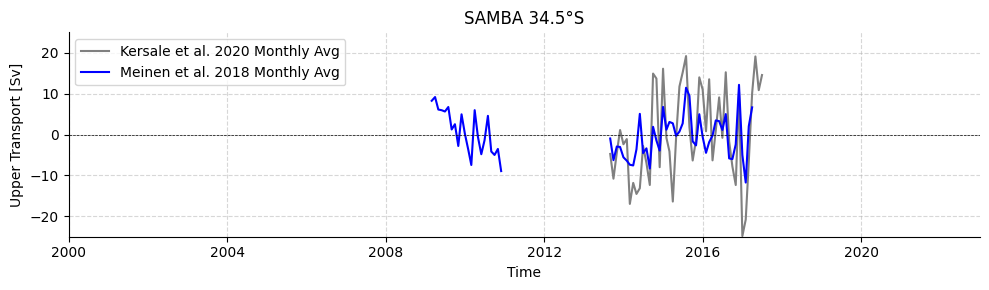
Load SAMBA 34.5°S
If you want to load all datasets available for a datasource, provide the option all_files=True. Note that the first time you do this, it will download the data for you. On subsequent runs (set up from the same location) it will use the previously downloaded data.
See the data reports in the docs: https://amoccommunity.github.io/AMOCatlas/ if you want to check how big a dataset is before downloading it.
[8]:
standardSAMBA = read.samba(all_files=True)
Loading 2 SAMBA 34.5°S dataset(s):
  0. Upper_Abyssal_Transport_Anomalies.txt: Daily volume transport anomaly estimates for the upper and abyssal cells of the MOC
  1. MOC_TotalAnomaly_and_constituents.asc: Daily travel time values, calibrated to a nominal pressure of 1000 dbar, and bottom pressures from the two PIES/CPIES moorings
[9]:
# Plot SAMBA timeseries
plotters.plot_amoc_timeseries(
    data=[standardSAMBA[0], standardSAMBA[1]],
    varnames=["UPPER_TRANSPORT", "MOC"],
    labels=["Kersale et al. 2020", "Meinen et al. 2018"],
    colors=["grey", "blue"],
    title="SAMBA 34.5°S",
    time_limits=("2000-01-01", "2022-12-31"),
    ylim=(-25, 25),
    resample_monthly=True,
    plot_raw=False # Raw data is a little spiky
)
[9]:
(<Figure size 1000x300 with 1 Axes>,
 <Axes: title={'center': 'SAMBA 34.5°S'}, xlabel='Time', ylabel='Upper Transport (Sv)'>)
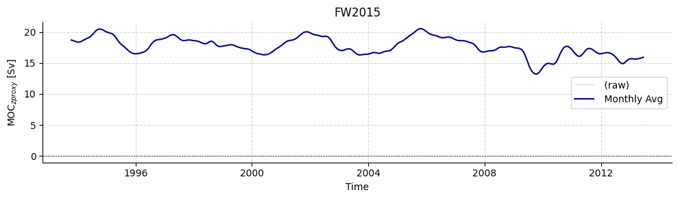
Load FW2015
For a formatted table showing the data including variables, dimensions, units etc, use the function plotters.show_variables(DATASET) where DATASET is an xarray dataset.
[10]:
standardfw2015 = read.fw2015()
plotters.show_variables(standardfw2015)
Loading 1 Frajka-Williams 2015 dataset(s):
  0. MOCproxy_for_figshare_v1.0.mat: Time series of MOC

information is based on xarray Dataset
[10]:
| dims | units | comment | standard_name | dtype | |
|---|---|---|---|---|---|
| name | |||||
| MOC | TIME | Sverdrup | ocean_meridional_overturning_transport | float64 | |
| MOC_PROXY | TIME | Sverdrup | ocean_meridional_overturning_streamfunction | float64 | |
| SSHA | TIME | cm | Sea_surface_height_anomaly | float64 | |
| TIME | TIME | datetime64[ns] | time | datetime64[ns] | |
| TRANS_1100_3000 | TIME | Sverdrup | ocean_volume_transport_across_line | float64 | |
| TRANS_3000_5000 | TIME | Sverdrup | ocean_volume_transport_across_line | float64 | |
| TRANS_EKMAN | TIME | Sverdrup | ocean_volume_transport_across_line | float64 | |
| TRANS_EKMAN__GRID | TIME | Sverdrup | ocean_volume_transport_across_line | float64 | |
| TRANS_FC | TIME | Sverdrup | ocean_volume_transport_across_line | float64 | |
| TRANS_FC_GRID | TIME | Sverdrup | ocean_volume_transport_across_line | float64 | |
| TRANS_UMO | TIME | Sverdrup | ocean_volume_transport_across_line | float64 | |
| TRANS_UMO_PROXY | TIME | Sverdrup | ocean_volume_transport_across_line | float64 |
[11]:
# Plot timeseries
plotters.plot_amoc_timeseries(
    data=[standardfw2015],
    varnames=["MOC_PROXY"],
    labels=[""],
    colors=["darkblue"],
    resample_monthly=True,
    plot_raw=True,
    title="FW2015"
)
[11]:
(<Figure size 1000x300 with 1 Axes>,
 <Axes: title={'center': 'FW2015'}, xlabel='Time', ylabel='MOC$_{z proxy}$ (Sv)'>)
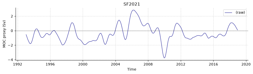
LOAD SANCHEZ-FRANKS 2021 26°N satellite reconstruction
[12]:
# Read dataset
standardsf2021 = read.sf2021()

# Show variables
plotters.show_variables(standardsf2021)
Loading 1 Sanchez-Franks et al. 2021 dataset(s):
  0. altimetry_moc_transport_1993_2020_18mos_smoothed.nc: A satellite reconstruction of the AMOC transport at 26N

information is based on xarray Dataset
[12]:
| dims | units | comment | standard_name | dtype | |
|---|---|---|---|---|---|
| name | |||||
| MOC_PROXY | TIME | Sverdrup | ocean_meridional_overturning_streamfunction | float64 | |
| TIME | TIME | datetime64[ns] | time | datetime64[ns] | |
| TRANS_GS_PROXY | TIME | Sverdrup | ocean_volume_transport_across_line | float64 | |
| TRANS_UMO_PROXY | TIME | Sverdrup | ocean_volume_transport_across_line | float64 |
[13]:
# Plot timeseries
plotters.plot_amoc_timeseries(
    data=[standardsf2021],
    varnames=["MOC_PROXY"],
    labels=[""],
    colors=["darkblue"],
    resample_monthly=False,
    #plot_raw=True,
    title="SF2021")
[13]:
(<Figure size 1000x300 with 1 Axes>,
 <Axes: title={'center': 'SF2021'}, xlabel='Time', ylabel='MOC proxy (Sv)'>)
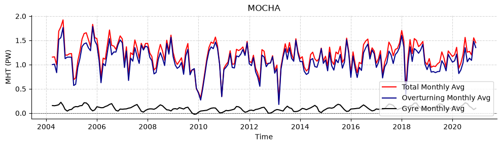
LOAD MOCHA 26.5°N
Note that AMOCatlas renames variables and updates units according to defaults specified in the code. For the MOCHA dataset, for example, the meridional heat transport is denoted by “Q”, whereas for other datasets it is “MHT”. To simplify intercomparison, we rename heat transport variables to “MHT”. When you use the read.mocha() this variable remapping has already taken place.
You can check the remapping applied in the docs: https://amoccommunity.github.io/AMOCatlas/
Additionally, some units such as “W” for Watts are converted to PetaWatts “PW” during the loading and standardisation. If instead you want to load the raw data, you can use read.mocha(raw=True).
[14]:
standardMOCHA = read.mocha()

plotters.show_variables(standardMOCHA)
Loading 1 MOCHA 26°N dataset(s):
  0. Johns_2023_mht_data_2020_ERA5.zip: No description available

information is based on xarray Dataset
/home/runner/work/AMOCatlas/AMOCatlas/amocatlas/reader_utils.py:83: SerializationWarning: Unable to decode time axis into full numpy.datetime64[ns] objects, continuing using cftime.datetime objects instead, reason: dates out of range. To silence this warning use a coarser resolution 'time_unit' or specify 'use_cftime=True'.
  ds = xr.open_dataset(file_path, **kwargs)
[14]:
| dims | units | comment | standard_name | dtype | |
|---|---|---|---|---|---|
| name | |||||
| MHT | TIME | PW | northward_ocean_heat_transport | float64 | |
| MHT_EKMAN | TIME | PW | northward_ocean_heat_transport_component | float64 | |
| MHT_FC | TIME | PW | northward_ocean_heat_transport_component | float64 | |
| MHT_GYRE | TIME | PW | as classically defined (e.g. see Johns et al., 2011). | northward_ocean_heat_transport_due_to_gyre | float64 |
| MHT_INT | TIME | PW | This only represents the contribution by the zonal mean v and T | northward_ocean_heat_transport_component | float64 |
| MHT_MO | TIME | PW | (Q_int + Q_wedge + Q_eddy) | northward_ocean_heat_transport_component | float64 |
| MHT_OT | TIME | PW | as classically defined (e.g. see Johns et al., 2011). | northward_ocean_heat_transport_due_to_meridional_overturning | float64 |
| MHT_WEDGE | TIME | PW | northward_ocean_heat_transport_component | float64 | |
| MOC | TIME | Sverdrup | ocean_meridional_overturning_transport | float64 | |
| Q_eddy | TIME | PW | derived from an objective analysis of interior ARGO T/S data merged with the mooring T/S data from moorings, and smoothly merged into the EN4 climatology along 26.5°N below 2000m. Q_eddy is not dependent on the temperature reference | northward_ocean_heat_transport_component | float64 |
| TEMP_FC_FWT | TIME | degree_C | sea_water_potential_temperature | float64 | |
| TIME | TIME | datetime64[ns] | time | datetime64[ns] | |
| TRANS_EKMAN | TIME | Sverdrup | ocean_volume_transport_across_line | float64 | |
| TRANS_FC | TIME | Sverdrup | from the cable | ocean_volume_transport_across_line | float64 |
| DEPTH | depth | m | depth | float64 | |
| TEMP_BASIN_MEAN | depth | degree_C | sea_water_potential_temperature | float64 | |
| TRANSPROF_BASIN_MEAN | depth | Sverdrup/m | northward_sea_water_velocity | float64 | |
| TRANSPROF_FC_MEAN | depth | Sverdrup/m | northward_sea_water_velocity | float64 | |
| STREAMFUNCTION_Z | string | Sverdrup | ocean_meridional_overturning_streamfunction | float64 | |
| TEMP_BASIN | string | degree_C | sea_water_potential_temperature | float64 | |
| TRANSPROF_BASIN | string | Sverdrup/m | northward_sea_water_velocity | float64 | |
| TRANSPROF_FC | string | Sverdrup/m | northward_sea_water_velocity | float64 |
[15]:
rawMOCHA = read.mocha(raw=True)
plotters.show_variables(rawMOCHA)
/home/runner/work/AMOCatlas/AMOCatlas/amocatlas/reader_utils.py:83: SerializationWarning: Unable to decode time axis into full numpy.datetime64[ns] objects, continuing using cftime.datetime objects instead, reason: dates out of range. To silence this warning use a coarser resolution 'time_unit' or specify 'use_cftime=True'.
  ds = xr.open_dataset(file_path, **kwargs)
/home/runner/work/AMOCatlas/AMOCatlas/amocatlas/plotters.py:276: SerializationWarning: Unable to decode time axis into full numpy.datetime64[ns] objects, continuing using cftime.datetime objects instead, reason: dates out of range. To silence this warning use a coarser resolution 'time_unit' or specify 'use_cftime=True'.
  "dtype": str(var.dtype) if isinstance(data, str) else str(var.data.dtype),
Loading 1 MOCHA 26°N dataset(s):
  0. Johns_2023_mht_data_2020_ERA5.zip: No description available

information is based on xarray Dataset
[15]:
| dims | units | comment | standard_name | dtype | |
|---|---|---|---|---|---|
| name | |||||
| T_basin_mean | depth | degree_C | float64 | ||
| V_basin_mean | depth | 1e6 m2 s-1 | float64 | ||
| V_fc_mean | depth | 1e6 m2 s-1 | float64 | ||
| z | depth | m | depth | float64 | |
| T_basin | string | degree_C | float64 | ||
| V_basin | string | 1e6 m2 s-1 | float64 | ||
| V_fc | string | 1e6 m2 s-1 | float64 | ||
| moc | string | 1e6 m3 s-1 | float64 | ||
| Q_eddy | time | W | derived from an objective analysis of interior ARGO T/S data merged with the mooring T/S data from moorings, and smoothly merged into the EN4 climatology along 26.5°N below 2000m. Q_eddy is not dependent on the temperature reference | float64 | |
| Q_ek | time | W | float64 | ||
| Q_fc | time | W | float64 | ||
| Q_gyre | time | W | as classically defined (e.g. see Johns et al., 2011). | float64 | |
| Q_int | time | W | This only represents the contribution by the zonal mean v and T | float64 | |
| Q_mo | time | W | (Q_int + Q_wedge + Q_eddy) | float64 | |
| Q_ot | time | W | as classically defined (e.g. see Johns et al., 2011). | float64 | |
| Q_sum | time | W | float64 | ||
| Q_wedge | time | W | float64 | ||
| T_fc_fwt | time | degree_C | float64 | ||
| day | time | float64 | |||
| hour | time | float64 | |||
| julian_day | time | object | |||
| maxmoc | time | 1e6 m3 s-1 | float64 | ||
| month | time | float64 | |||
| time | time | time | datetime64[ns] | ||
| trans_ek | time | 1e6 m3 s-1 | float64 | ||
| trans_fc | time | 1e6 m3 s-1 | from the cable | float64 | |
| year | time | float64 |
[16]:
rawMOCHA
[16]:
<xarray.Dataset> Size: 122MB
Dimensions:       (time: 12202, depth: 307)
Coordinates:
  * time          (time) datetime64[ns] 98kB 2004-04-02 ... 2020-12-14T12:00:00
Dimensions without coordinates: depth
Data variables: (12/26)
    Q_eddy        (time) float64 98kB 5.69e+13 5.509e+13 ... 6.124e+13 6.103e+13
    Q_ek          (time) float64 98kB -1.455e+14 -1.618e+14 ... 8.344e+14
    Q_fc          (time) float64 98kB 2.154e+15 2.18e+15 ... 2.335e+15 2.34e+15
    Q_gyre        (time) float64 98kB 1.355e+14 1.346e+14 ... 1.029e+14
    Q_int         (time) float64 98kB -1.668e+15 -1.665e+15 ... -1.87e+15
    Q_mo          (time) float64 98kB -1.414e+15 -1.408e+15 ... -1.697e+15
    ...            ...
    z             (depth) float64 2kB 5.995e+03 5.976e+03 ... 19.87 0.0
    julian_day    (time) object 98kB 8666-05-10 00:00:00 ... 8683-01-21 12:00:00
    year          (time) float64 98kB 2.004e+03 2.004e+03 ... 2.02e+03 2.02e+03
    month         (time) float64 98kB 4.0 4.0 4.0 4.0 ... 12.0 12.0 12.0 12.0
    day           (time) float64 98kB 2.0 2.0 3.0 3.0 ... 13.0 13.0 14.0 14.0
    hour          (time) float64 98kB 0.0 12.0 0.0 12.0 ... 0.0 12.0 0.0 12.0
Attributes: (12/23)
    comment:                       Dataset accessed and processed via http://...
    data_product:                  MOCHA heat transport at 26.5°N
    variable_mapping:              {'time': 'TIME', 'maxmoc': 'MOC', 'moc': '...
    convert_to_coord:              z
    variables_to_remove:           ['day', 'hour', 'julian_day', 'month', 'ye...
    original_variable_metadata:    {'Q_eddy': {'long_name': 'MHT_EDDY', 'desc...
    ...                            ...
    DOI:                           n/a
    Methodology reference:         W.E. Johns, S. Elipot, D.A. Smeed, B. Moat...
    Methodology DOI:               doi: 10.1098/rsta.2022.0188
    source_file:                   mocha_mht_data_ERA5_v2020.nc
    source_path:                   /home/runner/.amocatlas_data/mocha_mht_dat...
processing_datasource: mocha26n[17]:
# Plot timeseries
fig, ax = plotters.plot_amoc_timeseries(
    data=[standardMOCHA,standardMOCHA,standardMOCHA],
    varnames=["MHT", "MHT_OT","MHT_GYRE"],
    labels=["Total", "Overturning","Gyre"],
    colors=["red","darkblue","black"],
    resample_monthly=True,
    plot_raw=False,
    title="MOCHA"
)
ax.legend(loc="lower right")
[17]:
<matplotlib.legend.Legend at 0x7f3bee268050>
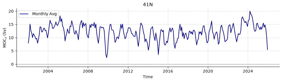
LOAD 41°N
Besides array-based datasets, some additional data sources are integrated within AMOCatlas. For instance, the Willis and Hobbs estimates of heat transport at 41°N and the Willis transport estimates using Argo and altimetry are available as datasource “WH41N”.
[18]:
file_list = read.wh41n.list_files()
print("Available WH41N files:")
print(file_list)

standard41n = read.wh41n()

plotters.plot_amoc_timeseries(
    data=[standard41n],
    varnames=["MOC"],
    labels=[""],
    resample_monthly=True,
    plot_raw=False,
    colors=["darkblue"],
    title="41N"
)
Available WH41N files:
['hobbs_willis_amoc41N_tseries.txt', 'trans_ARGO_ERA5.nc', 'Q_ARGO_obs_dens_2000depth_ERA5.nc']
Loading 1 Willis & Hobbs 41°N dataset(s):
  0. hobbs_willis_amoc41N_tseries.txt: Transport time series of Ekman volume, Northward geostrophc, Meridional Overturning volume and Meridional Overturning Heat
[18]:
(<Figure size 1000x300 with 1 Axes>,
 <Axes: title={'center': '41N'}, xlabel='Time', ylabel='MOC$_{z}$ (Sv)'>)
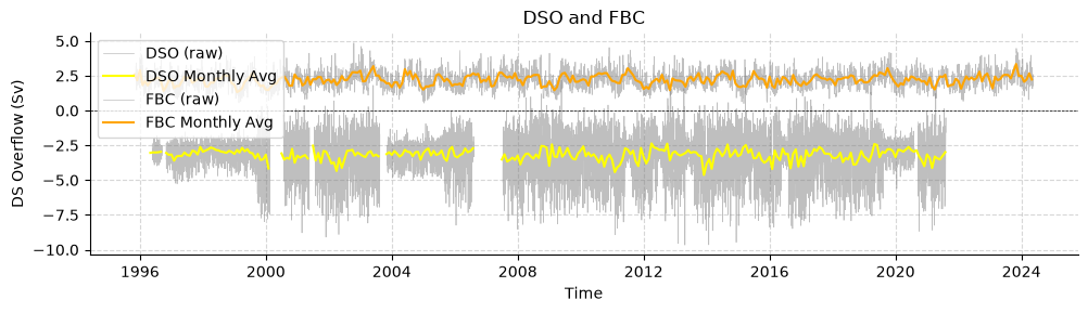
Load Denmark Strait overflow and Faroe Bank Channel overflow transports
Overflow transports for Denmark Strait and Faroe Bank Channel are also available.
Note that in the current version of AMOCatlas we have not standardised the sign of the transports. In this case, a stronger DSO is more negative, whereas a stronger FBC is more positive.
[19]:
standardDSO = read.dso()
standardFBC = read.fbc()

plotters.plot_amoc_timeseries(
    data=[standardDSO, standardFBC],
    varnames=["TRANS_DSO","TRANS_FBC"],
    labels=["DSO", "FBC"],
    resample_monthly=True,
    plot_raw=True,
    colors=["yellow", "orange"],
    title="DSO and FBC"
)
Loading 1 Denmark Strait Overflow dataset(s):
  0. DSO_transport_hourly_1996_2021.nc: Overflow time-series through Denmark Strait

Loading 1 Faroe Bank Channel dataset(s):
  0. OS_GSR_FBC_D_1995_2024.nc: Daily average of FBC overflow transport, estimated from an array of moored ADCPs in Sv
[19]:
(<Figure size 1000x300 with 1 Axes>,
 <Axes: title={'center': 'DSO and FBC'}, xlabel='Time', ylabel='DS Overflow (Sv)'>)
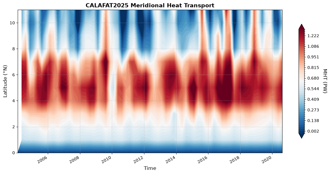
Load Calafat2025
Meridional heat transport from a Bayesian method to produce a North Atlantic heat budget is also available. However, it has 4000 realisations of the time series (from which uncertainties can be estimated), so is less straightforward to plot. See below for an average across the realisations.
[20]:
standardCALAFAT2025 = read.calafat2025()
standardCALAFAT2025
Loading 1 Calafat et al. 2025 dataset(s):
  0. Bayesian_estimates_Atlantic_MHT.zip: No description available
[20]:
<xarray.Dataset> Size: 49MB
Dimensions:     (lat: 12, TIME: 67, N_ENSEMBLE: 4000, number_regions: 11,
                 bound: 2)
Coordinates:
    LATITUDE    (lat) float64 96B 65.0 60.0 55.0 45.0 ... -5.0 -11.0 -25.0 -35.0
  * TIME        (TIME) datetime64[ns] 536B 2004-02-14T23:59:59.999996901 ... ...
  * N_ENSEMBLE  (N_ENSEMBLE) int64 32kB 0 1 2 3 4 5 ... 3995 3996 3997 3998 3999
    LAT_BOUNDS  (lat, bound) float64 192B 67.5 62.5 62.5 ... -30.0 -30.0 -40.0
Dimensions without coordinates: lat, number_regions, bound
Data variables:
    MHT         (lat, TIME, N_ENSEMBLE) float64 26MB ...
    HTC         (number_regions, TIME, N_ENSEMBLE) float64 24MB ...
Attributes: (12/39)
    title:                                 Observation-based probabilistic es...
    summary:                               MHT estimates dataset
    description:                           MHT estimates dataset
    program:                               Calafat2025
    project:                               Estimates of Atlantic meridional h...
    license:                               CC-BY-4.0
    ...                                    ...
    original_variable_metadata:            {'posterior_samples': {'long_name'...
    applied_variable_mapping:              {'mht': 'MHT', 'htc': 'HTC', 'post...
    creation data:                         31-Jul-2025 15:14:49
    contact:                               francisco.mcalafat@uib.eu
    comment on temporal resolution:        Estimates of heat transport are qu...
convections: CF-1.8, ACDD-1.3[21]:
def create_ensemble_mean_dataset(ds):
    """Create a new dataset with ensemble means, removing N_ENSEMBLE dimension.

    This function takes the mean across the N_ENSEMBLE dimension for all variables
    that have it, creating a dataset suitable for standard plotting functions.

    Parameters
    ----------
    ds : xarray.Dataset
        Input dataset with N_ENSEMBLE dimension

    Returns
    -------
    xarray.Dataset
        Dataset with ensemble means, N_ENSEMBLE dimension removed

    """
    # Create a copy of the dataset
    ds_mean = ds.copy()

    # For each data variable, take the mean across N_ENSEMBLE if it has that dimension
    for var_name in ds.data_vars:
        var = ds[var_name]
        if 'N_ENSEMBLE' in var.dims:
            # Take mean across N_ENSEMBLE dimension (point estimate)
            ds_mean[var_name] = var.mean(dim='N_ENSEMBLE')

    # Remove N_ENSEMBLE coordinate since no variables use it anymore
    if 'N_ENSEMBLE' in ds_mean.coords:
        ds_mean = ds_mean.drop_vars('N_ENSEMBLE')

    return ds_mean
[22]:
# Create the ensemble-averaged dataset
calafat_mean = create_ensemble_mean_dataset(standardCALAFAT2025)

# Now your original plotting code will work:
lat_idx = 5
lat_val = calafat_mean['LATITUDE'].values[lat_idx]

if lat_val<0:
    title_str = f'CALAFAT2025 (lat = {-lat_val:.2f}°S)'
else:
    title_str = f'CALAFAT2025 (lat = {lat_val:.2f}°N)'

  # Plot the 2D MHT data
fig, ax = plotters.plot_amoc_2d_data(
    data=calafat_mean,
    varname="MHT",
    title="CALAFAT2025 Meridional Heat Transport",
    ylabel="Latitude (°N)",
    figsize=(12, 6),
    colormap="RdBu_r",  # Red-blue colormap, good for heat transport
    # vmin=-1.0,  # Optional: set color scale limits
    # vmax=1.0,
)

# Add colorbar label
cbar = fig.get_axes()[1] if len(fig.get_axes()) > 1 else None
if cbar:
    cbar.set_ylabel('MHT (PW)', rotation=270, labelpad=20)
Load Zheng2024
Freshwater transports also available.
[23]:
# load ZHENG2024 dataset
standardZHENG2024 = read.zheng2024()

# create mean by using function defined for calafat2025 dataset earlier
zheng_mean = create_ensemble_mean_dataset(standardZHENG2024)

# Plot the 2D MFT data
fig, ax = plotters.plot_amoc_2d_data(
    data=zheng_mean,
    varname="MFT",
    title="ZHENG2024 Meridional Freshwater Transport",
    ylabel="Latitude (°N)",
    figsize=(12, 6),
    colormap="RdBu_r",  # Red-blue colormaps
    # vmin=-1.0,  # Optional: set color scale limits
    # vmax=1.0,
)

# Add colorbar label
cbar = fig.get_axes()[1] if len(fig.get_axes()) > 1 else None
if cbar:
    cbar.set_ylabel('MFT (Sv)', rotation=270, labelpad=20)
Loading 1 Zheng et al. 2024 dataset(s):
  0. atl_mft_2000_extend_gpcp_oaflux.nc: An observation-based estimate of the Atlantic meridional freshwater transport
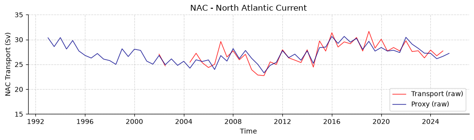
Load NAC timeseries
Available for plotting is a transport estimate by satellite and float observations (TRANS_NAC) and a proxy only based on satellite altimetry (TRANS_NAC_PROXY). Both are shown here.
Dataset is already in 6-monthly resolution, which is why the raw data is shown in the plot. If you type resample_monthly = False then the raw data is shown in your desired color.
[24]:
# Load dataset
standardNAC = read.nac()
Loading 1 North Atlantic Current, M. Lankhorst, 2025 dataset(s):
  0. _2_1.nc: 6-monthly estimates of NAC transport from satellite altimetry and float observations
[25]:
fig, ax = plotters.plot_amoc_timeseries(
    data=[standardNAC,standardNAC],
    varnames=["TRANS_NAC", "TRANS_NAC_PROXY"],
    labels=["Transport", "Proxy"],
    colors=["red","darkblue"],
    resample_monthly=False,
    plot_raw=True,
    title="NAC - North Atlantic Current",
    ylim=(15, 35),
)
ax.legend(loc="lower right") # Plot NAC transport and proxy timeseries
[25]:
<matplotlib.legend.Legend at 0x7f3bedcd8ad0>
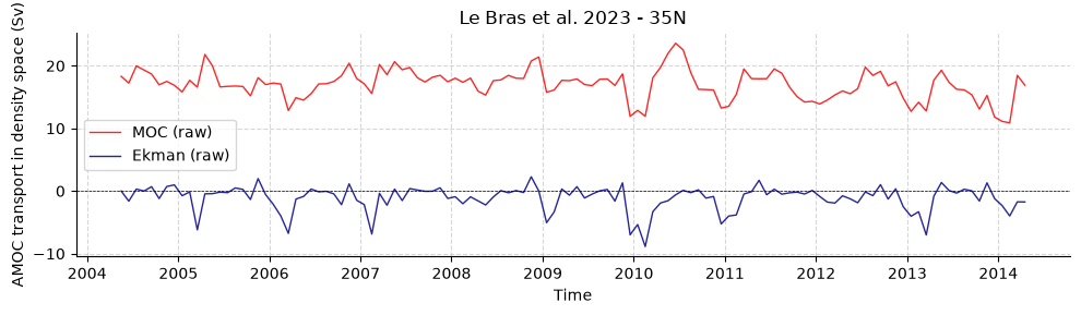
Load Le Bras 35°N AMOC
[26]:
# Load dataset
# This dataset has multiple files, so we specify all_files=True create a list of datasets.
# They can then be accessed with standardLEBRAS35N[0] (transport data) and standardLEBRAS35N[1] (gridded velocities).
# If you only want the transport files, you could specify: transport_only=True
standardLEBRAS35N = read.lebras35n(all_files=True)
Loading 2 Le Bras et al. 2023 at 35°N dataset(s):
  0. AMOC35N.nc: AMOC transport data at 35°N
  1. AMOC35N_gridded_velocities.nc: Gridded velocity data through the section at 35°N
[27]:
# Plot MOC and Ekman component of transport timeseries
# In the plot the data is displayed as (raw) because it is already on a monthly grid, so no resampling was needed.
plotters.plot_amoc_timeseries(
    data=[standardLEBRAS35N[0],standardLEBRAS35N[0]],
    varnames=["MOC_SIGMA2", "TRANS_EKMAN"],
    labels=["MOC", "Ekman"],
    resample_monthly=False,
    plot_raw=True,
    colors=["red", "darkblue"],
    title="Le Bras et al. 2023 - 35N"
)
[27]:
(<Figure size 1000x300 with 1 Axes>,
 <Axes: title={'center': 'Le Bras et al. 2023 - 35N'}, xlabel='Time', ylabel='AMOC transport in density space (Sv)'>)
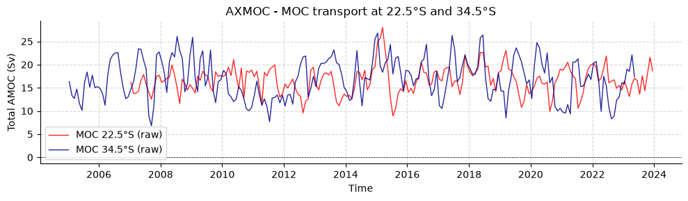
Load the AXMOC transport data for 22.5°S and 34.5°S
use read.axmoc22s() for the 22.5°S data (here we have MOC and MHT available)
use read.axmoc34s() for the 34.5°S data (here we have MOC, MHT and FOV available) (FOV = overturning component of freshwater transport)
For both datasets we have the total, then the Ekman and the geostrophic component available
[28]:
standardAXMOC22S = read.axmoc22s()
standardAXMOC34S = read.axmoc34s()
Loading 1 AXMOC 22.5°S dataset(s):
  0. AXMOC_22S_timeseries_2007_2023.nc: AMOC and MHT transport data at 22.5°S

Loading 1 AXMOC 34.5°S dataset(s):
  0. AXMOC_34S_timeseries_2005_2023.nc: AMOC, MHT and FOV transport data at 34.5°S
[29]:
plotters.plot_amoc_timeseries(
    data=[standardAXMOC22S,standardAXMOC34S],
    varnames=["MOC", "MOC"],
    labels=["MOC 22.5°S", "MOC 34.5°S"],
    resample_monthly=False,
    plot_raw=True,
    colors=["red", "darkblue"],
    title="AXMOC - MOC transport at 22.5°S and 34.5°S"
)
[29]:
(<Figure size 1000x300 with 1 Axes>,
 <Axes: title={'center': 'AXMOC - MOC transport at 22.5°S and 34.5°S'}, xlabel='Time', ylabel='Total AMOC (Sv)'>)
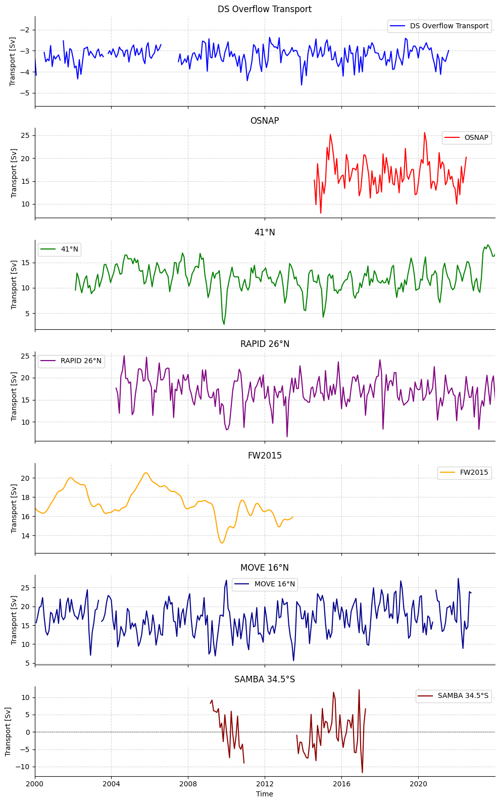
Monthly Anomalies Overview
[30]:
plotters.plot_monthly_anomalies(
    osnap_data=ds_osnap["MOC_SIGMA0"],
    fortyone_data = standard41n["MOC"],
    rapid_data=standardRAPID[0]["MOC"],
    move_data=-ds_move["MOC"],
    samba_data=standardSAMBA[1]["MOC"],
    fw2015_data=standardfw2015["MOC_PROXY"],
    dso_data = standardDSO["TRANS_DSO"],
    osnap_label="OSNAP",
    fortyone_label = "41°N",
    rapid_label="RAPID 26°N",
    move_label="MOVE 16°N",
    samba_label="SAMBA 34.5°S",
    fw2015_label="FW2015",
    dso_label = "DS Overflow Transport"
)
[30]:
(<Figure size 1000x1600 with 7 Axes>,
 array([<Axes: title={'center': 'DS Overflow Transport'}, ylabel='Transport (Sv)'>,
        <Axes: title={'center': 'OSNAP'}, ylabel='Transport (Sv)'>,
        <Axes: title={'center': '41°N'}, ylabel='Transport (Sv)'>,
        <Axes: title={'center': 'RAPID 26°N'}, ylabel='Transport (Sv)'>,
        <Axes: title={'center': 'FW2015'}, ylabel='Transport (Sv)'>,
        <Axes: title={'center': 'MOVE 16°N'}, ylabel='Transport (Sv)'>,
        <Axes: title={'center': 'SAMBA 34.5°S'}, xlabel='Time', ylabel='Transport (Sv)'>],
       dtype=object))

Other components
It is also possible to manipulate (filter) and plot other components of the AMOC, depending on what is available in the datasets.
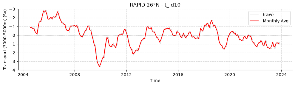
[31]:
clim = standardRAPID[0].groupby("TIME.month").mean("TIME")
tmp = standardRAPID[0].groupby("TIME.month") - clim
filtRAPID = tmp.rolling(TIME = 500, center = True).mean()

fig,ax = plotters.plot_amoc_timeseries(
    data=[filtRAPID],
    varnames=["TRANS_3000_5000"],
    labels=[""],
    resample_monthly=True,
    plot_raw=True,
    title="RAPID 26°N - t_ld10"
)
ax.set_ylim(4, -3)

fig.show()